Tag: Excel

Lock Cells in Excel Mastering Protection

Lock Cells in Excel is a powerful technique for protecting your spreadsheet data. It allows you to prevent accidental changes, creating secure and user-friendly worksheets. This guide will walk you through various methods for locking cells, from basic protection to advanced password-locking and specific cell range controls. Learn how to safeguard your data and create professional-looking spreadsheets.

Whether you’re building financial reports, inventory trackers, or complex data models, locking cells can significantly improve data integrity. We’ll explore practical applications and troubleshoot potential problems, ensuring you master this essential Excel skill.

Introduction to Locking Cells in Excel

Locking cells in Excel is a powerful technique to protect specific data from accidental modification. It’s a crucial feature for maintaining data integrity and consistency within spreadsheets, especially in collaborative environments. This method allows you to designate certain cells as read-only, preventing users from unintentionally altering their contents.By strategically locking cells, you can safeguard formulas, important calculations, and critical data entry points, leading to more reliable and accurate spreadsheets.

This control over cell modification contributes to improved data quality and reduces the likelihood of errors.

Defining Locking Cells

Locking cells in Excel means preventing users from changing the values, formulas, or formatting of designated cells. These cells remain fixed and cannot be modified, providing a degree of protection.

Purpose and Benefits of Locking Cells

Locking cells is essential for maintaining data accuracy and consistency. By restricting modifications, you can safeguard critical data points, ensuring that only authorized individuals or groups can alter them. This is especially useful in shared spreadsheets where multiple users might be working on the same document.

Protecting a Worksheet vs. Locking Cells

Protecting a worksheet is a broader security measure that locks the entire worksheet, preventing any modifications. Locking cells, however, provides more granular control. You can choose which cells to lock and which to leave unlocked, offering a tailored level of protection. This allows for a greater degree of flexibility in controlling access to specific information within a worksheet.

Common Scenarios for Locking Cells

Locking cells is highly useful in various situations. For example, in financial reports, locking cells containing pre-defined formulas prevents accidental changes that could compromise the accuracy of the calculations. Similarly, in data entry forms, locking cells used for summary calculations protects the data integrity of the final report. Moreover, in shared spreadsheets, locking cells containing constants or look-up values ensures that everyone uses the same, correct data.

Basic Example of Locked and Unlocked Cells

This table illustrates the concept of locked and unlocked cells. The table displays data that is protected by locking certain cells, while others remain modifiable. This demonstrates the granular control afforded by locking cells within a spreadsheet.

Column A (Locked)	Column B (Unlocked)
2023 Sales Target	Sales Rep
$1,000,000	John Smith
$1,200,000	Jane Doe
$1,500,000	David Lee

In this example, Column A (containing sales targets) is locked, preventing users from changing these values. Column B (containing sales representatives) is unlocked, allowing users to update this information. This separation of modifiable and non-modifiable data provides a clear visual distinction for data protection.

Methods for Locking Cells

Securing specific cells in your Excel spreadsheets is crucial for maintaining data integrity and preventing accidental modifications. This article details various methods for locking cells, enabling you to protect sensitive information and enforce data consistency. Understanding these techniques empowers you to create more robust and reliable spreadsheets.

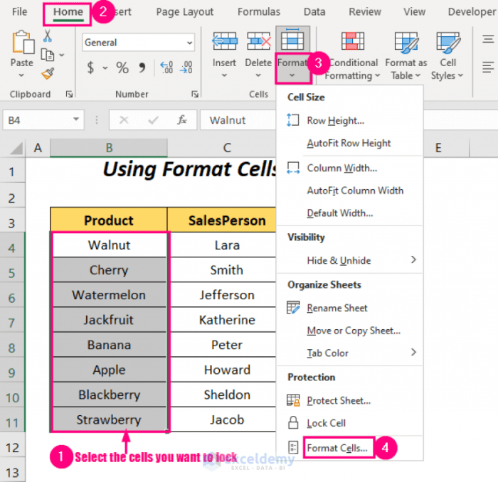
Using the Format Cells Option

This method allows you to lock individual cells directly. Select the cells you want to protect. Right-click and choose “Format Cells.” Navigate to the “Protection” tab. Check the “Locked” box. This locks the cells, preventing any changes to their values.

Crucially, remember that locking a cell does not automatically protect it; a sheet protection step is still required.

Protecting the Sheet

Protecting a sheet is a fundamental step to enforce the locking of cells. After locking cells using the Format Cells option, you must protect the sheet. Select “Review” on the Excel ribbon. Click “Protect Sheet.” Enter a password (optional but highly recommended) to safeguard the protection. Specify which cells or ranges should be locked by selecting “Locked cells.” This prevents users from changing protected cells, even if they are allowed to edit the rest of the sheet.

Locking Cells with VBA

Visual Basic for Applications (VBA) offers a powerful and flexible way to lock cells programmatically. This method is ideal for complex scenarios or automated tasks. VBA code allows you to specify the cells to lock dynamically, making it well-suited for large datasets or recurring tasks. You can use VBA to lock specific cells in a sheet, or to control the locking of cells based on certain conditions or events.“`VBASub LockCells() Dim rng As Range Set rng = Range(“A1:B5”) ‘Specify the range to lock With rng .Locked = True .Interior.Color = vbYellow End With ActiveSheet.Protect DrawingObjects:=False, Contents:=True, Scenarios:=False, Password:=”mypassword”End Sub“`This example locks cells A1 through B5 and highlights them in yellow.

The password is crucial to protect the locked cells from unauthorized access.

Comparison of Methods

Method	Description	Pros	Cons
Format Cells	Locks cells individually	Simple for single cell locking	Not suitable for complex locking schemes.
Protect Sheet	Enforces locking of cells after locking with Format Cells	Easy to implement, good for basic protection	Can be cumbersome for advanced protection.
VBA	Dynamic locking via code	Highly flexible, suitable for complex logic	Requires VBA knowledge

This table summarizes the key characteristics of each method, aiding in the selection of the most appropriate technique for your specific needs. Choosing the right method depends on the complexity of your spreadsheet and the level of protection you require.

Advanced Locking Techniques: Lock Cells In Excel

Mastering cell locking in Excel goes beyond basic protection. Advanced techniques allow for more granular control, ensuring data integrity and preventing unintended modifications. This involves password protection, targeted cell range locking, and handling formulas and charts within the locked structure. These methods provide a more robust security layer for your spreadsheets.

Password Protection for Locked Cells

Password protection adds an extra layer of security to locked cells. This prevents unauthorized access even if the worksheet is unlocked. It is crucial for sensitive data. Enter the password when setting the protection and again whenever you need to modify the protected cells.

Locking Specific Cell Ranges

Locking specific cell ranges allows for greater control over protected areas. Instead of locking the entire worksheet, you can select and protect only the cells containing crucial data, maintaining flexibility for other, non-sensitive areas. This ensures that only designated cells are restricted.

Locking Cells Containing Formulas

Formulas, crucial parts of spreadsheets, can be locked to prevent unintended changes to their logic. Locking these cells maintains the integrity of calculations. This is especially important for complex models and financial projections where formula alterations could lead to inaccurate results.

Learning to lock cells in Excel is super helpful for creating spreadsheets that stay organized. It’s a fundamental skill, like knowing how to design your dream Sims home in The Sims 4. Make Sims Inspired in The Sims 4 is a great resource if you want to design some cool characters! Once you master locking cells, you can prevent accidental changes, making your spreadsheets much more reliable.

This is crucial for maintaining accurate data.

Locking Cells That Are Part of a Chart

Locking cells that are part of a chart is essential for maintaining data consistency. Protecting the data source cells ensures that any changes reflected in the chart accurately represent the underlying data. This is important when updating the source data without affecting the chart’s integrity.

Example: Password Protection and Cell Range Locking

The following example demonstrates password protection and cell range locking in a practical scenario. It uses a simple HTML table to represent the spreadsheet.

Product	Price	Quantity
Product A
Product B

The price and quantity cells are locked. These values cannot be directly modified by users. This ensures that the underlying data used for the chart remains consistent and unchanged.

To lock the cells in the table, select the cells, right-click, and choose “Format Cells”. Then select the “Protection” tab and check the “Locked” box. To apply password protection, go to “Review” > “Protect Sheet”.

Important Note: This example uses HTML table representation. Actual Excel implementation will involve the Excel application’s tools and functions for cell locking and password protection.

Practical Applications of Locked Cells

Locking cells in Excel offers significant advantages beyond basic protection. It empowers users to create robust spreadsheets that prevent accidental modifications, ensuring data integrity and consistency. This is crucial for collaborative projects, user-friendly forms, and protected templates, ultimately enhancing the overall security of the spreadsheet.By understanding how to lock cells, you can design spreadsheets that are not only functional but also resilient to errors and misuse.

This control extends beyond simple protection, enabling more complex functionalities like user-specific data entry and customized reporting.

Locking cells in Excel is crucial for protecting data, especially when collaborating. It’s like creating a safe zone for specific parts of your spreadsheet. Just like how Kendrick Lamar’s DNA gets a new version for the NBA finals, this new twist on the NBA Finals theme requires some carefully considered adjustments. Knowing which cells to lock ensures your data stays secure and avoids accidental edits, keeping your spreadsheets organized and your work efficient.

Preventing Accidental Data Modification

Accidental changes to critical data can lead to errors and wasted time. Locked cells provide a crucial safeguard against this. Imagine a spreadsheet tracking financial data; if certain cells containing formulas or predefined values are locked, users cannot inadvertently alter these critical elements, thus maintaining the integrity of the calculations. This feature is vital for preventing errors and maintaining data accuracy in collaborative environments.

Creating User-Friendly Forms

Locked cells are essential for designing user-friendly forms in Excel. A form for collecting customer information, for example, could lock cells that automatically calculate totals or contain pre-defined formulas. Users can then input data into specific fields without inadvertently altering the calculations or format of the form. This approach makes the form straightforward and intuitive to use, ensuring data accuracy and consistency.

Creating Protected Templates

Locked cells are vital for creating protected templates. Consider a template for invoices. Locking the cells containing headers, formulas for calculating amounts, or predetermined formatting ensures that users cannot change the structure or calculations of the template. This ensures that all invoices adhere to the required format and calculations, maintaining consistency and accuracy.

Enhancing Data Security

Locking cells is a fundamental step in data security. By locking cells containing sensitive information, you restrict access to those values. For example, a spreadsheet with confidential financial data could lock all cells containing sensitive financial figures. This method significantly strengthens the security of the spreadsheet, preventing unauthorized modifications and ensuring the confidentiality of the data.

Locking cells in Excel is a pretty handy feature, especially when you’re working with spreadsheets that need to be protected from accidental edits. It’s all about safeguarding data integrity. This reminds me of the recent initiative in the grand duchy, where the people are being given a voice, grand duchy let the people speak , a great example of how letting the public share their opinions can lead to better outcomes.

Ultimately, locking cells is about maintaining order and accuracy within the spreadsheet.

Visual Demonstration, Lock Cells in Excel

Application	Description	Example
Preventing Accidental Modification	Locking cells containing formulas or constant values to maintain data integrity.	A spreadsheet calculating employee salaries. The salary structure (basic pay, allowances) is locked, preventing users from altering these values.
Creating User-Friendly Forms	Locking cells containing formulas or pre-defined formatting to prevent unintended modifications.	A customer survey form with locked calculation fields. Users input data, and the form automatically calculates totals.
Creating Protected Templates	Locking cells containing headers, calculations, or formatting to maintain template consistency.	An invoice template with locked headers, calculation fields, and currency formatting.
Enhancing Data Security	Locking cells containing sensitive information to restrict unauthorized modifications.	A spreadsheet with confidential financial data. Cells containing account balances, transaction details, or sensitive information are locked.

Troubleshooting Common Issues

Locking cells in Excel can be a powerful tool, but it’s essential to understand how to address potential problems. Incorrect configurations or user errors can lead to unexpected results. This section details common issues encountered when working with locked cells, along with their solutions and preventative measures.Troubleshooting locked cells involves identifying the root cause of the problem and applying appropriate fixes.

Knowing how to unlock cells that are unintentionally locked is just as important as knowing how to lock them in the first place. By understanding the potential problems and their solutions, you can efficiently resolve any issues that arise.

Potential Problems and Solutions

Incorrect cell locking can stem from various factors. Understanding the configuration settings is crucial to avoid issues. Misconfigurations or simple errors can lead to unexpected behavior.

Locked cells preventing editing: If a cell is locked and you cannot edit it, verify the protection status for the worksheet. Ensure that the worksheet is protected and that the specific cells are locked. If protected, unlock the worksheet or modify the locked cells’ protection attributes. This involves checking the “Protect Sheet” option in the “Review” tab.
Error messages during locking: Excel may display error messages if the lock attempt violates worksheet protection settings. Common errors include “Cannot lock cells” or “Sheet protection is active.” These errors usually indicate a conflict between your locking action and the protection status of the sheet. Review the sheet protection settings, unlock the sheet if necessary, and then try locking the cells again.

Verify that the sheet is not protected or locked in another application.
Unintentional locking of necessary cells: Accidental locking of cells used for data entry can hinder workflow. Review the locked cells list and unlock those that are crucial for input. This can be done by using the “Unprotect Sheet” option in the “Review” tab to unlock all cells or selecting individual cells to unlock them. If you accidentally locked cells, use the “Unprotect Sheet” option in the “Review” tab to unlock the worksheet.

Then select the specific cells and uncheck the “Locked” box in the Format Cells dialog box.

Unlocking Locked Cells

Unlocking locked cells is straightforward. Follow these steps to revert a cell to its editable state.

Unprotect the worksheet: To unlock all cells, unprotect the worksheet using the “Unprotect Sheet” option in the “Review” tab. This will allow all cells to be edited without restrictions. This will also eliminate the need for further cell-specific unlocking.
Unlock specific cells: If only some locked cells need to be unlocked, select the cells and go to the “Format Cells” dialog box. Locate the “Protection” tab and uncheck the “Locked” option. Click “OK”. This method targets specific cells without affecting other parts of the worksheet.

Error Messages and Explanations

Different error messages can indicate various problems with locking cells. Understanding their meanings is crucial for efficient troubleshooting.

Error Message	Explanation
“Cannot lock cells”	This error suggests that the worksheet is currently protected. Unlock the worksheet to allow locking.
“Sheet protection is active”	The sheet protection settings are preventing you from locking cells. Unprotect the sheet to allow locking.
“You do not have permission to change the sheet protection.”	Insufficient user privileges. Contact the worksheet administrator or obtain appropriate permissions to modify protection settings.

Comparison of Locking Methods

Unlocking the power of Excel’s cell protection features involves choosing the right locking method. Different techniques cater to varying needs, offering varying levels of control and flexibility. Understanding the nuances of each approach is crucial for optimizing spreadsheet security and maintainability.Different methods for locking cells in Excel offer varying levels of protection and control. Choosing the right method depends on the specific requirements of your spreadsheet.

This comparison will explore the advantages and disadvantages of each approach, along with situations where one method is superior to another.

Protection Methodologies

Various methods are available for locking cells in Excel, each with its own set of characteristics. The most common methods involve using the worksheet’s protection feature, employing formulas, and implementing custom VBA code. Each method offers distinct advantages and disadvantages.

Worksheet Protection

Worksheet protection is a straightforward method for locking cells. It allows you to protect entire worksheets or specific ranges of cells, preventing accidental changes or modifications.

Advantages: Simplicity and ease of implementation are key advantages. It’s a quick way to secure a sheet or a range of cells from unintended alterations.
Disadvantages: Limited granular control over individual cells. You can’t easily restrict access to specific cells within a protected range. Requires the user to manually unprotect the sheet to make changes.

Using Formulas

Using formulas in conjunction with cell locking can provide more specific control over cell contents. Formulas can validate or calculate data within protected cells, limiting input possibilities.

Advantages: Enhanced data integrity by validating inputs and preventing invalid entries. Formulas can dynamically adjust cell values.
Disadvantages: Can become complex when implementing advanced validation rules. Requires a basic understanding of formulas.

Custom VBA Code

Custom VBA code offers the most granular control over cell locking. It allows for highly customized and complex scenarios, including complex data validation, advanced restrictions, and even dynamic locking based on specific conditions.

Advantages: Extremely flexible and allows for intricate control. Can automate locking and unlocking based on user interactions or other events. Offers the most fine-grained control.
Disadvantages: Requires a good understanding of VBA programming. Implementation can be more time-consuming compared to other methods.

Comparative Table

Locking Method	Advantages	Disadvantages	Suitable Situations
Worksheet Protection	Simple, easy to implement	Limited granular control, requires manual unprotect	Protecting entire sheets or specific ranges from accidental modification
Formulas	Data validation, dynamic calculations	Complexity for advanced validation, requires formula knowledge	Restricting inputs to specific values or calculations
Custom VBA Code	Highly flexible, granular control, automation	Requires VBA knowledge, time-consuming implementation	Complex scenarios, custom validation, dynamic locking based on conditions

Illustrative Examples

Unlocking the power of locked cells in Excel isn’t just about preventing accidental changes; it’s about ensuring data integrity and accuracy across various applications. This section provides practical examples of locking different cell types, showcasing their use in financial reports, inventory tracking, and other scenarios. We’ll see how locking cells can significantly improve data reliability and consistency.Understanding how to lock cells is crucial for maintaining the precision and reliability of your Excel spreadsheets.

By restricting edits to specific cells, you safeguard critical data, preventing errors and ensuring the integrity of your analyses.

Financial Reporting

Protecting formulas and constants in financial reports is paramount. Locked cells in this context act as safeguards, preventing unauthorized changes to key figures or calculations. This approach enhances the trustworthiness of your financial analyses.

Example: A spreadsheet for calculating monthly budgets. You want to lock cells containing the initial budget figures entered by management, while allowing for the input of actual spending figures in other cells.

Cell	Content	Locked?	Description
A1	2023 Budget (Sales)	Yes	Initial budget value, locked to prevent accidental changes.
A2	2023 Actual Sales	No	User input for the actual sales figure.
B1:B12	Monthly budget	Yes	Locked, preventing changes to the budget allocations.
B13	Total Budget	Yes	Formula-driven total, locked to maintain accuracy.

This example demonstrates how locking specific cells ensures that the initial budget figures remain unchanged while allowing adjustments to actual figures. This structure maintains data integrity, and avoids errors that might arise from accidentally altering the budget.

Inventory Tracking

In inventory management, locked cells can protect crucial data points like product codes, unit costs, and reorder levels. This approach ensures accuracy in stock calculations and minimizes errors in inventory reports.

Example: An inventory spreadsheet. You want to lock the product codes and their corresponding unit costs, allowing users to update quantities on hand and calculate values based on these locked parameters.

Cell	Content	Locked?	Description
A1:A10	Product Codes	Yes	Locked to prevent accidental changes to product identifiers.
B1:B10	Unit Costs	Yes	Locked, ensuring that the cost of each product remains consistent.
C1:C10	Quantity on Hand	No	User input for the current inventory level.
D1:D10	Calculated Value	No	Formula calculating the total value of each product based on quantity and cost.

By locking the product codes and unit costs, the integrity of the inventory data is maintained. This prevents accidental modification of these essential elements, and ensures that calculations are based on accurate values.

Customization and Design Considerations

Beyond the functionality of locked cells, enhancing their visual presentation significantly improves usability and readability within your Excel spreadsheets. Properly highlighting locked cells can prevent errors and confusion, especially in complex spreadsheets. This section explores various techniques to customize the appearance of locked cells, making them stand out and aid in comprehension.

Customizing Cell Appearance

The basic method of locking cells in Excel often leaves the locked cells indistinguishable from unlocked ones. This section focuses on techniques to make locked cells more prominent.

Highlighting Locked Cells

Different visual cues can effectively highlight locked cells. A simple yet effective approach is to apply a distinctive background color. For instance, a light yellow or a pale blue can clearly mark locked cells without overpowering the overall spreadsheet design. Another option is to use a different font color for the locked cells. A darker color, such as a dark navy blue or dark gray, will stand out against the standard font color.

Visual Cues for Enhanced Readability

To further enhance readability and comprehension, visual cues can be strategically added to locked cells. One method is to use a subtle border around the locked cells. A thin, contrasting border can visually separate locked cells from unlocked cells without being overly distracting. Consider using a different cell fill color, like a very light shade of green or a light orange.

A subtle, yet noticeable, border around the cell can significantly improve the visual separation of locked cells.

Creating a Responsive HTML Table

A responsive HTML table allows for dynamic adjustments based on screen size, ensuring optimal display on various devices. This is crucial for maintaining the visual appeal and readability of locked cells across different viewing environments. Below is an example of how you might implement this:

Cell Type	Background Color	Border	Font Color
Locked	Light Yellow	1px solid Dark Gray	Dark Blue
Unlocked	White	1px solid Light Gray	Black

This example uses a table to visually represent the different styling options for locked and unlocked cells. Adjusting the background colors, border styles, and font colors can be tailored to match the overall design of the spreadsheet. The table demonstrates how the style of locked cells can be easily customized to enhance the clarity of the spreadsheet.

Examples of User-Friendly Forms

Creating user-friendly forms is crucial for efficient data entry and reducing errors. Locking cells strategically in these forms ensures data integrity and prevents accidental modifications, especially important in shared environments or when dealing with sensitive information. These locked cells act as a safeguard, preventing unauthorized changes and maintaining the accuracy of the data.

Data Entry Forms with Locked Cells

Protecting data entry forms is essential. By locking specific cells, you can prevent users from inadvertently altering critical parts of the form. This ensures the accuracy and reliability of the collected information. For example, you might lock cells containing calculated values or pre-defined constants, preventing erroneous alterations.

Customer Order Form: A customer order form can have locked cells for customer ID, order date, and predefined product codes. These fields, often automatically populated or derived from other systems, should remain unchanged to maintain data consistency. Unlocking these fields only for authorized personnel ensures accurate and consistent data.
Employee Timesheet: In an employee timesheet, the employee ID and project code fields should be locked. These are pre-defined values and shouldn’t be altered by the employee. Only the hours worked and other modifiable fields should be unlocked for input.

Forms with Locked Headers and Calculated Fields

Forms with headers and calculated fields can benefit significantly from locked cells. This ensures that the form’s structure and pre-calculated data remain unchanged. Locking headers prevents accidental deletion or modification, preserving the form’s layout and integrity.

Item	Price	Total
Product A	$10.00	$10.00
Product B	$5.00	$10.00
Subtotal		$20.00

In the example table above, the header row (Item, Quantity, Price, Total) and the calculated “Total” column are locked. Users can only modify the quantity, and the total will automatically update based on the input, maintaining data integrity.

Responsive HTML Table for Forms

Using a responsive HTML table for forms enhances usability across various devices. The locked cells and calculated fields within this table remain consistent, regardless of screen size or device.

Product	Description	Price	Total
Product A	Description for Product A	$10.00	$10.00
Product B	Description for Product B	$5.00	$10.00
Subtotal			$20.00

The responsive HTML table ensures the form’s layout adapts to different screen sizes. The locked header and calculated fields maintain their integrity and position across various devices.

Closing Notes

In conclusion, mastering Lock Cells in Excel empowers you to create robust, secure, and user-friendly spreadsheets. By understanding the different locking methods, you can effectively protect your data from accidental modification, enhance data integrity, and streamline data entry processes. This comprehensive guide has provided a detailed overview of the entire process, from basic techniques to advanced password protection and customization.

Now you’re equipped to confidently use this vital Excel tool.

August 5, 2023

Label Axes in Excel Charting Clarity

Label Axes in Excel is crucial for creating insightful charts. Without clear labels, your visualizations can be confusing and misleading. This guide dives deep into the art of effectively labeling both X and Y axes, ensuring your Excel charts communicate data accurately and compellingly. From understanding fundamental axis concepts to mastering different chart types, we’ll explore the best practices for creating professional-looking charts that tell a story.

We’ll cover everything from basic labeling techniques to advanced customizations, like adjusting font sizes and using logarithmic scales. Learn how to craft concise and informative labels that clearly convey the data represented in your charts. Whether you’re creating bar charts, line graphs, or scatter plots, this guide provides the tools and insights to transform your Excel charts into powerful communication tools.

Introduction to Excel Axes

Excel charts are powerful tools for visualizing data. At the heart of these visualizations are the axes, which provide a framework for understanding the relationships between different variables. Properly labeled axes are crucial for accurate interpretation and effective communication of insights.Axes in Excel spreadsheets define the coordinate system for plotting data points. They establish the scale and units along which data values are represented.

Label axes, specifically, provide context by indicating the meaning of the values on each axis. This context is essential for anyone interpreting the chart’s information.

Fundamental Concept of Axes

Axes are the foundation of any chart. They establish the scale and units used to represent data. The horizontal axis (x-axis) typically represents the independent variable, while the vertical axis (y-axis) represents the dependent variable. Understanding this fundamental relationship is crucial for drawing meaningful conclusions from the chart.

Definition of Label Axes

Label axes means adding descriptive labels to the x-axis and y-axis to clearly indicate what the values represent. These labels are not just arbitrary names; they are critical for conveying the meaning of the data plotted on the chart. For example, an x-axis labeled “Time (hours)” instantly tells the viewer the units of the data along that axis.

Importance of Labeling Axes in Excel Charts

Clear axis labeling is vital for effective chart interpretation. Without proper labels, viewers might struggle to understand the data being presented. A chart with ambiguous labels can lead to misinterpretations, and even potentially erroneous conclusions. This highlights the importance of choosing descriptive and unambiguous labels for each axis.

How Incorrect Axis Labeling Affects Chart Interpretation

Incorrect or missing axis labels can significantly impact the comprehension of a chart. Consider a chart showing sales figures over time without specifying the time period. The viewer might not understand if the data represents sales over a week, a month, or a year. This lack of clarity can lead to misinterpretations and incorrect conclusions about the trends.

Example of an Excel Chart with Labeled Axes

Imagine a chart displaying the growth of a company’s revenue over a five-year period. The x-axis is labeled “Year (2018-2022)” and the y-axis is labeled “Revenue (USD in Millions)”. This clear labeling allows the viewer to immediately understand the context of the data. The chart’s title could further clarify the specific company or industry. A well-labeled chart, in this example, immediately conveys the company’s revenue growth from 2018 to 2022.

Figuring out how to label axes in Excel can be a real head-scratcher, but it’s a crucial skill for clear data visualization. While I was wrestling with Excel’s labeling functions, I decided to take a break and listen to some new music, like the latest track by Isaiah Rashad, SZA, and 6lack. This song really got me in the zone, and now I’m ready to tackle those Excel axes again.

Once you get the hang of labeling your axes, your charts will be so much more informative!

Different Chart Types and Axes

Excel’s charting capabilities extend far beyond simple bar graphs. Understanding the various chart types and their associated axes is crucial for effectively communicating data insights. Different chart types excel at showcasing different relationships and trends, and the axes play a vital role in accurately representing these data points. Choosing the appropriate chart type is critical for conveying the intended message.Different chart types employ axes in diverse ways, emphasizing specific aspects of the data.

The structure of these axes, and the way data is mapped onto them, significantly impacts how the chart conveys information. Understanding these nuances allows for the creation of charts that are both informative and easy to interpret.

Chart Types and Axis Structure

Various chart types in Excel leverage axes differently to highlight distinct data relationships. This section details how different chart types employ axes.

Bar Charts: Bar charts use categorical data on the horizontal axis (x-axis) and numerical data on the vertical axis (y-axis). The height of each bar directly corresponds to the value on the y-axis, making it easy to compare quantities across different categories. The x-axis labels often represent different categories or groups, while the y-axis represents the magnitude of the values.

Axis labels are critical for clarity and understanding the comparisons being made.
Line Charts: Line charts are effective for visualizing trends over time or continuous variables. The x-axis usually represents the independent variable (e.g., time), and the y-axis represents the dependent variable (e.g., sales). The lines connect data points, illustrating the changes in the dependent variable as the independent variable progresses. Clear axis labels are essential for interpreting the trend accurately.
Scatter Plots: Scatter plots depict the relationship between two numerical variables. Both the x-axis and y-axis represent numerical values. Each data point is plotted as a marker, and the pattern of the points reveals the correlation or lack thereof between the two variables. Precise axis scaling is crucial for accurately representing the relationship.

Impact of Chart Type on Axis Labeling

The choice of chart type influences the required detail and complexity of axis labeling. Clear and concise labels are paramount for accurate data interpretation.

Bar Charts: Bar chart labels should clearly identify the categories being compared. For example, instead of simply “Sales,” labels might specify “Sales by Region” or “Sales by Product Type.” The y-axis label should precisely describe the measured quantity, like “Sales in Dollars.”
Line Charts: Line chart labels need to clearly define the independent and dependent variables. For example, if the x-axis represents time, the label might be “Time in Months,” and the y-axis label could be “Sales Revenue.” Consistent units are essential for accuracy.
Scatter Plots: Scatter plot axis labels should precisely identify the variables being plotted. For example, labels like “Customer Age” and “Purchase Amount” ensure accurate interpretation of the relationship between the variables.

Different Axis Scales

Different chart types may require different axis scales to effectively represent the data.

Bar Charts: Scales should be appropriate for the range of values in the data, ensuring all bars are clearly visible and easily compared. Choosing a scale that allows for clear visualization of differences between bars is crucial.
Line Charts: Scales should accommodate the range of values and ensure that trends are clearly visible. Scales should be chosen to showcase the overall trends and not distort the data.
Scatter Plots: The scale should allow for the precise plotting of data points and the identification of any correlations or patterns. A logarithmic scale may be necessary if the data has a very wide range of values.

Chart Type and Axis Considerations Table

Chart Type	X-Axis	Y-Axis	Labeling Considerations
Bar Chart	Categorical Data	Numerical Data	Clear category labels, precise unit descriptions
Line Chart	Continuous Data (e.g., Time)	Numerical Data	Independent and dependent variable labels, consistent units
Scatter Plot	Numerical Data	Numerical Data	Precise variable labels, appropriate scale for data range

Labeling the X-axis

Effective X-axis labels are crucial for clear and accurate chart interpretation. They provide context and meaning to the data plotted on the horizontal axis, allowing viewers to understand the independent variable and its relationship to the dependent variable. A well-crafted X-axis label can significantly enhance the overall understanding and impact of your chart.Properly labeled X-axes transform raw data into meaningful insights.

They connect the visual representation to the underlying information, facilitating easier comprehension and informed decision-making. This section dives into best practices for crafting informative and effective X-axis labels in Excel charts.

Effective X-axis Label Examples

Different types of data require different label styles. A label for sales figures over time should differ from one depicting product categories. Examples of effective labels include “Time (Years)”, “Product Category”, “Temperature (°C)”, or “Sales (USD)”. Notice how these labels clearly communicate the data’s nature and units.

Figuring out how to label axes in Excel can be tricky, but it’s essential for clear visualizations. While you’re wrestling with those axis labels, why not take a break and listen to Nicki Minaj and Ariana Grande’s new song, “Bed” listen to nicki minaj and ariana grandes new song bed ? Once you’ve got your groove on, come back to Excel and ensure your charts are easily understandable with properly labeled axes.

It’s all about making data shine!

Creating Concise and Informative Labels

To create concise and informative labels, avoid unnecessary jargon or overly technical terms. Use clear and straightforward language that the intended audience can easily grasp. For example, instead of “Quarterly Revenue Growth Rate,” opt for “Sales Growth (Qtr.)”. Keep the label brief and focused on conveying the essential information. Conciseness enhances readability and reduces clutter.

Formatting X-axis Labels

Font size and alignment are critical formatting elements. A font size that is too small makes the label difficult to read, while a size that is too large can overcrowd the chart. Font size should be proportionate to the overall chart size and text. Center alignment is often the most effective choice for labels, ensuring they are clearly visible and easily readable.

Importance of Units in X-axis Labels

Always include appropriate units in your X-axis labels. This ensures clarity and accuracy. For example, if the data represents time in months, the label should read “Time (Months)”. If the data represents temperature, the label should specify the unit of measurement, such as “Temperature (°C)”. Omitting units can lead to misinterpretations and inaccuracies in data analysis.

Table of X-axis Label Formats

Label Format	Effectiveness	Explanation
Sales (2022-2024)	Good	Clearly indicates the time period for sales data.
Time (Years)	Excellent	Provides a generic but informative description.
Product Type (Q1 2023)	Fair	Needs additional context; consider specifying the year.
Revenue (Qtrly)	Poor	Lacking clarity on units (currency).
Temperature (Celsius)	Excellent	Specifies the measurement unit for temperature.

This table demonstrates the importance of including units and clear time periods. A clear label helps avoid misunderstandings and promotes effective data interpretation.

Labeling the Y-axis: Label Axes In Excel

Effective labeling of the Y-axis is crucial for clear and accurate data representation in Excel charts. A well-defined Y-axis allows the audience to quickly grasp the magnitude and trends of the data being presented. This is vital for conveying information effectively and avoiding misinterpretations. Properly labeled axes empower viewers to draw meaningful conclusions from the data.Precise and unambiguous labeling of the Y-axis is paramount to ensure the data presented is accurately interpreted.

This involves selecting appropriate units, ranges, and formats to ensure that the relationship between the values on the Y-axis and the corresponding data points is readily understood. A poorly labeled Y-axis can lead to misinterpretations and a failure to grasp the true story behind the data.

Strategies for Effective Y-Axis Labeling

Careful consideration of the Y-axis scale is vital for accurate data representation. The choice of scale greatly impacts how the data is perceived. A linear scale is suitable for data that shows a consistent rate of change, while a logarithmic scale is beneficial for data with large variations or exponential growth.

Specifying Units for the Y-Axis, Label Axes in Excel

Explicitly stating the units associated with the Y-axis values is essential for proper data interpretation. This avoids ambiguity and ensures that viewers understand the context of the data. For example, if the Y-axis represents sales figures, including the unit “dollars” (e.g., “Sales (USD)”) clarifies the meaning of the values. Without units, the values become abstract and meaningless.

Figuring out how to label axes in Excel can be a real pain sometimes, but it’s a crucial step for clear visualizations. It’s like setting up a clean slate, especially when you’re dealing with a lot of data. This is analogous to wiping a Mac clean, Wipe a Mac Clean , which is useful when you need a fresh start for your computer.

Ultimately, properly labeling your Excel axes makes your charts much easier to understand and interpret.

Examples of Effective Y-Axis Labels

Here are some examples of effective Y-axis labels:

Population (Thousands): This label clearly indicates that the Y-axis values represent population figures, and the use of “thousands” provides context for the scale.
Profit Margin (%): This label specifies that the Y-axis values represent profit margins expressed as percentages, which is essential for accurate interpretation.
Temperature (°C): This label specifies the unit of measurement for the Y-axis, temperature in degrees Celsius, making the data instantly understandable.

Avoiding Ambiguity in Y-Axis Labels

Ambiguity in Y-axis labels can lead to misinterpretations. For example, a label simply reading “Sales” is insufficient without specifying the units (e.g., “Sales (USD)”) or the time period covered. A clear and concise label, using appropriate units and providing context, is crucial for accurate interpretation. The label should directly correspond to the data being plotted.

Formatting Y-Axis Labels, Including Logarithmic Scales

The formatting of Y-axis labels significantly impacts readability and clarity. Use clear and easily readable fonts, and ensure the labels are not overlapping with other chart elements. Consider using logarithmic scales when dealing with data exhibiting significant variations in magnitude. A logarithmic scale compresses the large values, allowing for a more comprehensive visualization of trends across a wide range of data.

Linear Scale: This is suitable for data where values change consistently. The scale increases in equal increments along the Y-axis.
Logarithmic Scale: This scale is particularly useful when dealing with data that spans several orders of magnitude. It compresses large values, allowing for a more comprehensive visualization of trends across a wider range of data. A logarithmic scale is useful for data that exhibits exponential growth or decay.

Customizing Axis Labels

Taking your Excel charts from basic to beautiful involves customizing axis labels. This crucial step allows you to enhance readability, convey specific information, and tailor the chart to your exact needs. Clear and well-formatted labels are essential for effective communication through charts.Modifying axis labels in Excel is a straightforward process, allowing you to control various aspects of their appearance, from the font and color to their alignment and format.

This flexibility empowers you to create visually appealing and informative charts.

Modifying Axis Label Text

To change the text displayed on your axis labels, select the axis you want to modify. Then, right-click on the axis label. This will open a context menu offering options to modify the label text. Alternatively, you can click on the label itself, and the formatting options should be available in the ribbon. This allows for direct editing of the label’s content, whether it’s a simple change or a complete rewrite.

Customizing Font, Color, and Size

Once you’ve selected the axis label, look for the “Font” options in the formatting section of the ribbon. Here, you can change the font style, size, and color. Select the desired font, adjust the font size to an appropriate level for readability, and choose a color that complements the chart’s theme. Using bold fonts can highlight critical data points or axis labels.

Darker colors on a light background, or vice versa, generally ensure better visibility.

Rotating and Aligning Axis Labels

Excel allows for rotation and alignment of axis labels for optimal readability. You can rotate labels to prevent overlapping and enhance clarity. Adjusting the label alignment, such as left, center, or right, ensures labels are aligned with the data they represent, enhancing the overall aesthetics and clarity of the chart. This adjustment is particularly helpful when dealing with labels that contain longer text strings.

Using Custom Number Formats

Custom number formats allow for more sophisticated presentation of axis labels, especially when dealing with numerical data. For example, you can format labels to display currency, percentages, or dates in a specific style. This feature ensures data is presented in a way that’s both informative and visually appealing.For example, you can use a custom format to display percentages with a “%” symbol appended, or to show dates in a specific order (e.g., MM/DD/YYYY).

This formatting will automatically adjust the labels based on the corresponding data.

Example: Formatting Axis Labels for Readability

Let’s say you have a chart showing sales figures over time. You could use a custom number format to display the sales figures as currency (e.g., “$1,234”). You could also use a bold, dark blue font for the labels, ensuring high visibility against a light-colored background. This combination will make the chart easily readable and instantly convey the financial information.

Rotating the labels by a few degrees can also be useful in avoiding overlaps.

Ending Remarks

In conclusion, mastering axis labeling in Excel is a vital skill for anyone working with data visualization. By understanding the importance of clear and informative labels, you can transform your charts from static displays into dynamic communication tools. This guide has provided a comprehensive overview of the different aspects of labeling axes, from basic concepts to advanced customization techniques.

Remember, clear labels are key to effective data communication. By applying the techniques discussed here, you can significantly enhance the clarity and impact of your Excel charts.

August 1, 2023